by Timo Niemann
> This report will be a bit more 'well defined' ## Reproducibility > '-' means use the last non '-' left value | Reproducibility factor | Task 1 value | Task 2 value | Task 3 value | Task 4.1 value | Task 4.2 value | Task 5.1 value | Task 5.2 value | |:---|:---:|:---:|:---:|:---:|:---:|:---:|:---:| | MATLAB Version | 26.1.0.3251617 (R2026a) Update 2 | - | - | - | - | - | - | | 5G Toolbox Version | 26.1 | - | - | - | - | - | - | | WLAN Toolbox Version | 26.1 | - | - | - | - | - | - | | Communications Toolbox Version | 26.1 | - | - | - | - | - | - | | Parallel Computing Toolbox Version | 26.1 | - | - | - | - | - | - | | Random stream | mt19937ar with seed | - | - | - | - | - | - | | Random seed | 666 | - | - | - | - | - | - | | SNR vector | $0:1:40\,dB$ | - | - | - | - | - | $30\,dB$ | | Packet budget | 1024 packets per SNR point | - | - | - | - | - | 1 representative packet per profile | | maxNumErrors | 50 | - | - | - | - | - | 1 | | NTN profile | NTN-TDL-C | - | - | - | - | NTN-TDL-A to NTN-TDL-D | - | | Carrier frequency | 2.4 GHz | - | Task 3.2: [1 2.4 5 5.8 6 12 24 60] GHz | - | - | 2.4 GHz | - | | LEO altitude | 600 km | - | - | - | - | - | - | | Elevation sequence | 10° to 90° to 10° over the packet sequence | - | - | - | - | - | first packet of the sequence, 10° | | Mean elevation angle | 50° | - | - | - | - | - | not averaged, 10° representative packet | | Mean slant range | 906.32 km | - | - | - | - | - | not averaged, 10° representative packet | | Mean satellite Doppler shift | 32.73 kHz | - | changes with carrier frequency | - | - | 32.73 kHz | not averaged, 10° representative packet | | Normalized CFO | 0.419 | - | changes with carrier frequency | - | - | 0.419 | not averaged, 10° representative packet | | Channel bandwidth | 20 MHz | - | - | - | [20 40 80 160 320] MHz | 20 MHz | 320 MHz | | MCS | 2 | - | - | [0 2 4 8 10 12 13] | 3 | 2 | - | | APEP length | 1000 B | [250 1000 4000 8000 12000] B | Task 3.1: [250 1000 4000 8000 12000] B; Task 3.2: 8000 B | - | - | 1000 B | - | | TX/RX antennas | 1-by-1 SISO | - | - | - | - | - | - | | Pilot tracking | disabled | - | enabled | - | - | disabled | - | | Parallelization | parfor over SNR points | - | - | - | - | parfor over SNR points per profile | parfor over NTN profiles | ## Task1 #### 1.1 See code `lab_4.m`, `create_baseline_configuration.m` and `simulateTransmission.m`. #### 1.2  The plot shows the packet error rate significantly decreasing as the signal to noise ration increases. This behavior can be observed when the SNR reaches a value of 25, at that simulation point the signal significantly overweights the noise and the PER also significantly decreases in an negative exponential manner. At link level, PER is the fraction of transmitted PHY-layer packets that are not received correctly for a given channel model and SNR. #### 1.3 For the baseline configuration with $f_c = 2.4GHz$, LEO altitude $600km$, orbital shifted elevation angle (Elevation sequence: 10° to 90° to 10° over the packet sequence, mean: $50°$), and static receiver. The mean slant range is $906.32km$, the computed mean satellite Doppler shift is approximately $32.73kHz$. With the IEEE $802.11be$ subcarrier spacing of $78.125kHz$, this corresponds to a normalized CFO of $\epsilon \approx 0.419$. Therefore, the Doppler shift is below one subcarrier spacing but still represents $41.9%$ of the OFDM subcarrier spacing. #### 1.4 ##### CFR Magnitude single representative Packet:  The CFR magnitude of the representative packet is relatively flat over the active subcarriers. Only moderate variations are visible, without deep frequency-selective fades. Therefore, for the baseline 20 MHz NTN-TDL-C configuration, the channel appears mostly frequency-flat to mildly frequency-selective. ##### Complete CFR Magnitude over all representative Packets by first MCS:  The complete CFR collection is included as a consistency check. The collected packet CFRs show similar magnitude variations over the active subcarriers, indicating that the selected representative packet is typical for this baseline run. No strong deep fades are visible across most packets, so the 20 MHz NTN-TDL-C baseline appears mostly frequency-flat to mildly frequency-selective. ## Task 2 #### 2.1  ###### Visual analysis: The PER-over-SNR curves shift to higher SNR values for larger APEP values. In contrast to the other graphs APEP = 250 B has the highest rate of successful transmitted packets. ###### Analyzing by meaning: Smaller APEP values perform better than larger APEP values. In particular, APEP = 250 B reaches low PER at lower SNR than the larger payload sizes. As the payload size increases, the plot shifts to the right, so larger packets need a higher SNR to achieve the same packet error rate. Using a small APEP results in more successfully transmitted packets, but also increases the needed network usage / protocol overhead, more smaller packets mean more packet headers, resulting in more data that needs to be transferred in sum. Increasing APEP increases the number of payload bits and therefore the number of EHT-Data OFDM symbols. Larger APEP increase the packet duration. Since pilot tracking is disabled, residual CFO and common phase error are not continuously corrected during the data field. The longer the packet lasts, the more residual phase error can accumulate, which increases the probability that the packet is decoded incorrectly. The residual CFO is more harmful to longer packets because the phase error accumulates over the packet duration. ###### Summary: Increasing APEP increases the number of payload bits and therefore the number of EHT-Data OFDM symbols. This increases the packet duration. Since pilot tracking is disabled, residual CFO and common phase error are not continuously corrected during the data field. The longer the packet lasts, the more residual phase error can accumulate, which increases the probability that the packet is decoded incorrectly. #### 2.2 | Target PER | Reasonable SNR | Practical maximum APEP | |:---:|:---:|:---:| | $10^{-1}$ | $23\,dB$ | $600\,B$ | The target PER for this task is $10^{-1}$. I use $23\,dB$ as a practical SNR limit, because it is close to the beginning of the low-PER region while still avoiding the very high-SNR tail of the simulation. From the focused APEP comparison, APEP $= 600\,B$ reaches PER $\leq 10^{-1}$ at approximately $23\,dB$. Larger payloads require a higher SNR to reach the same target PER. Therefore, under the chosen practical SNR limit, APEP $= 600\,B$ is selected as the practical maximum payload size. 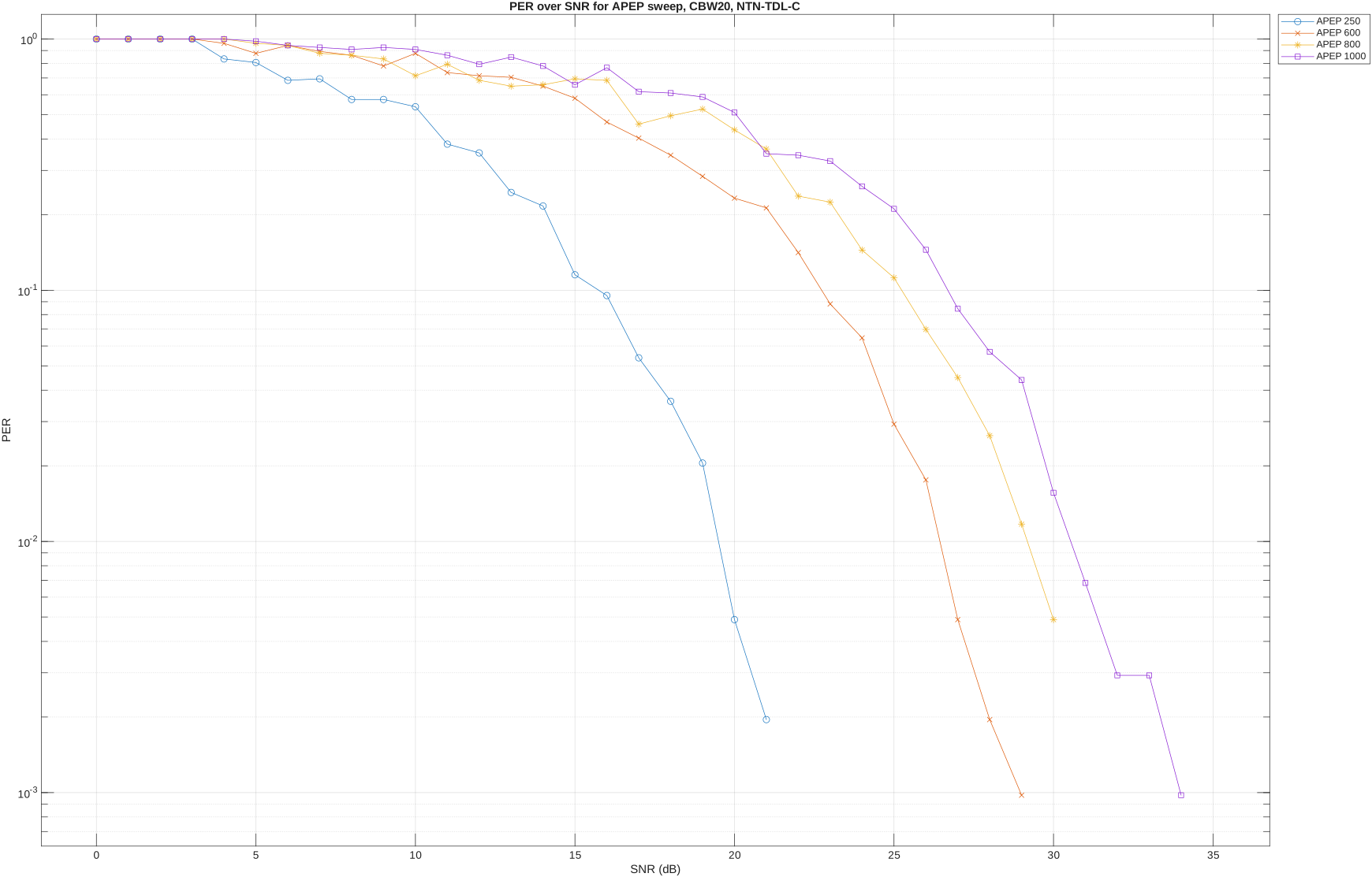 This choice is a compromise between robustness and overhead. Smaller packets such as APEP $= 250\,B$ are more robust, but require more packets and therefore more protocol overhead to transmit the same amount of user data. Larger packets reduce overhead, but are more sensitive to residual CFO because of their longer packet duration. As a practical motivation, this SNR limit can be interpreted as a conservative design choice for difficult deployment scenarios, for example remote or terrain-challenged areas. This was not explicitly simulated in this lab, since the channel model does not include blockage, vegetation, or terrain shadowing. However, such scenarios often involve small battery-powered devices with limited energy availability. Therefore, choosing a payload size that reaches the target PER without relying on the very high-SNR tail is useful, because it leaves more link margin and can reduce the need for retransmissions. In this sense, APEP = 600 B is a practical compromise between robustness, packet overhead, and energy-aware operation. For applications where higher data rates are more important than robustness, a larger payload such as APEP $= 4000\,B$ may still be attractive because it reduces relative packet overhead. In the simulated range, this requires operating closer to the high-SNR end of the sweep, approximately around $40\,dB$ for the target PER. ## Task 3 #### 3.1 ##### Full Task 2 APEP Plot with pilot tracking enabled: 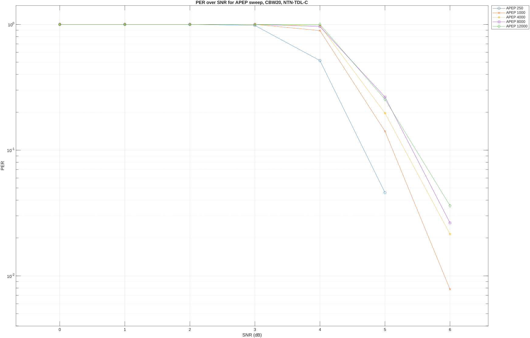 ##### Comparision plot with APEP = 4000 B: 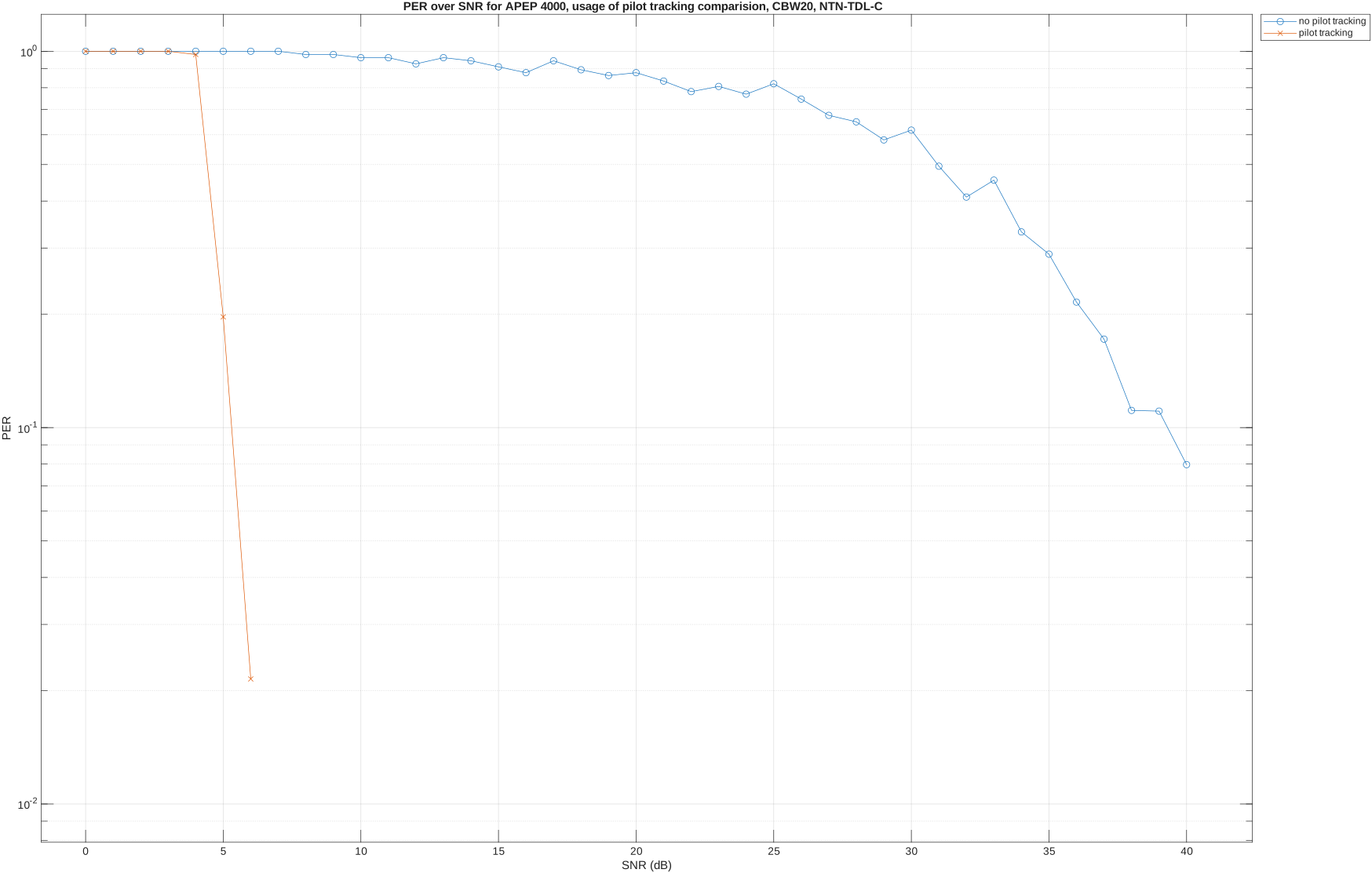 Comparing the plots shows a significant improvement when pilot tracking is enabled. Pilot tracking uses the EHT-Data pilots to compensate residual common phase error during the data field. This is especially beneficial for larger packets, because residual CFO has more time to accumulate phase error over the packet duration. For APEP = 4000 B, the target PER of $10^{-1}$ is reached at approximately $5.25\,dB$ with pilot tracking, compared to approximately $40\,dB$ without pilot tracking. This shows that pilot tracking strongly improves CFO tolerance for long packets. #### 3.2 ##### PER over SNR Frequency sweep without pilot tracking: 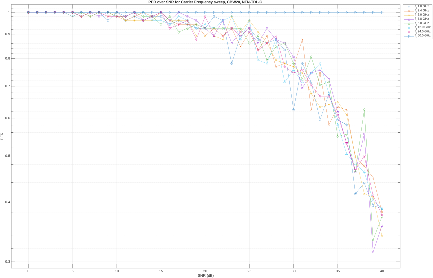 ##### PER over SNR Frequency sweep with pilot tracking: 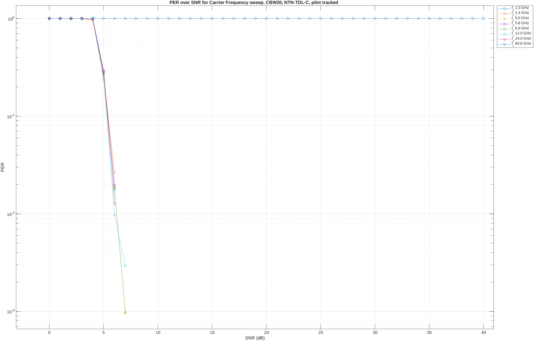 | Frequency | Mean Doppler Shift | Normalized Carrier Frequency Offset epsilon |:---:|:---:|:---:| | 1.0 GHz | ~13.64kHz | ~0.17 | | 2.4 GHz | ~32.73kHz | ~0.42 | | 5.0 GHz | ~68.19kHz | ~0.87 | | 5.8 GHz | ~79.11kHz | ~1.01 | | 6.0 GHz | ~81.83kHz | ~1.05 | | 12.0 GHz | ~163.67kHz | ~2.09 | | 24.0 GHz | ~327.33kHz | ~4.19 | | 60.0 GHz | ~818.33kHz | ~10.47 | The carrier-frequency sweep shows the linear dependency between carrier frequency and satellite-induced Doppler shift. At 1 GHz the mean Doppler shift is only about 13.64 kHz, corresponding to a normalized CFO of epsilon = 0.17. At the baseline frequency of 2.4 GHz, the normalized CFO increases to about 0.42. Around 5.8 GHz, epsilon reaches approximately 1, meaning that the Doppler shift is already on the order of one 802.11be subcarrier spacing. The higher-frequency stress cases become much more severe: at 12 GHz epsilon is about 2.09, at 24 GHz about 4.19, and at 60 GHz about 10.47. This explains why the PER performance degrades for higher carrier frequencies. A larger normalized CFO causes stronger common phase rotation and inter-carrier interference. Pilot tracking improves the result because it uses the EHT-Data pilots to compensate residual common phase error during the data field. However, for very large CFO values, especially the stress case at 60 GHz, pilot tracking cannot compensate the impairment because the offset is already several subcarrier spacings. $\textbf{Pilot tracking}$ shifts the PER curves to lower SNR and makes longer packets and higher carrier frequencies more robust. Its benefit is strongest when the receiver can still perform packet detection and preamble-based CFO correction, but residual phase error remains during the EHT-Data field. If the CFO becomes too large, pilot tracking alone is not sufficient. #### 3.3 Based on the simulated carrier frequency sweep, 6 GHz can be considered a practical upper carrier frequency for the tested Wi-Fi 7 NTN setup when pilot tracking is enabled. At 6 GHz, the normalized CFO is approximately $\epsilon = 1.05$, which means that the Doppler shift is already close to one OFDM subcarrier spacing. Nevertheless, the PER curve with pilot tracking still remains usable compared to the higher frequency stress cases. The frequencies above 6 GHz show a much stronger impairment. At 12 GHz, 24 GHz, and 60 GHz, the normalized CFO becomes several subcarrier spacings, so pilot tracking alone can be no longer sufficient to fully compensate the doppler induced frequency offset. Within the simulated setup, 6 GHz is selected as a practical limit because it is still inside the Wi-Fi 7 frequency range and remains manageable with pilot tracking. However, this conclusion is based on the fixed 20 MHz simulation bandwidth and the resulting lab data and without real world application. The possible real world advantage of the 6 GHz band, such as more available spectrum and wider channels, is not directly evaluated here. #### 3.4 At very low SNR, pilot tracking can have little visible impact because the receiver is limited by noise. The pilot subcarriers are also corrupted by noise, so the residual common phase error estimate becomes unreliable. Packet detection, synchronization, and data demodulation errors dominate the PER. In this region, correcting residual CFO does not help much because the packet is already limited by the low SNR. #### 3.5 At very high SNR, pilot tracking can also have little visible impact because the receiver may already recover most packets after packet detection and coarse/fine CFO correction. The PER is then close to zero, so there is little room for pilot tracking to visibly improve the curve. Meaning the link is no longer limited by noise and the remaining residual phase error is small enough for the receiver. For extreme carrier frequency stress cases, the CFO can be so large that pilot tracking alone is insufficient. This is a separate limitation caused by doppler rather than low noise. ## Task 4 #### 4.1 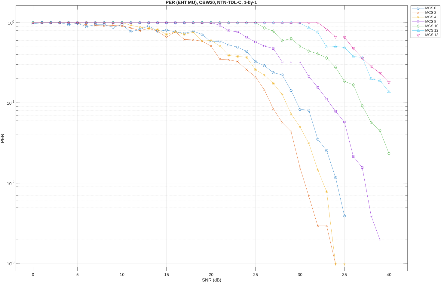 The MCS sweep shows that higher MCS values require higher SNR to achieve the same packet error rate. Lower MCS values are more robust and can reach PER values around $10^{-3}$ within the simulated SNR range, but this comes at the cost of a lower data rate. For MCS 12 and MCS 13, the PER does not fall below $10^{-1}$ in the observed SNR range. In particular, MCS 13 still shows a high packet error rate around 34 dB SNR where as MCS 0 reaches PER $10^{-3}$, so it is not reliable under these channel conditions. Reflecting this analysis: Higher MCS values tend to be more sensitive to NTN Doppler and residual CFO. #### 4.2 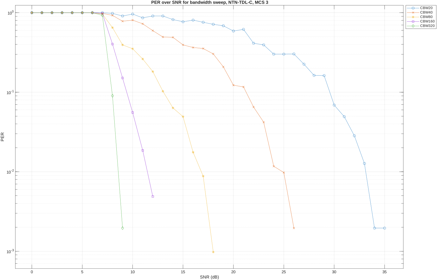 Analyzing the bandwidth sweep, the observed PER improves as the channel bandwidth increases. In this simulation setup, CBW320 reaches a PER of approximately nearly $10^{-3}$ below 10 dB SNR, while CBW20 requires roughly 34-35 dB SNR to reach a comparable PER. This indicates that, for the fixed APEP length and MCS used here, a wider channel bandwidth improves the link robustness in the simulated NTN channel. So in this simulation a higher bandwith improves PER. ## Task 5 #### 5.1 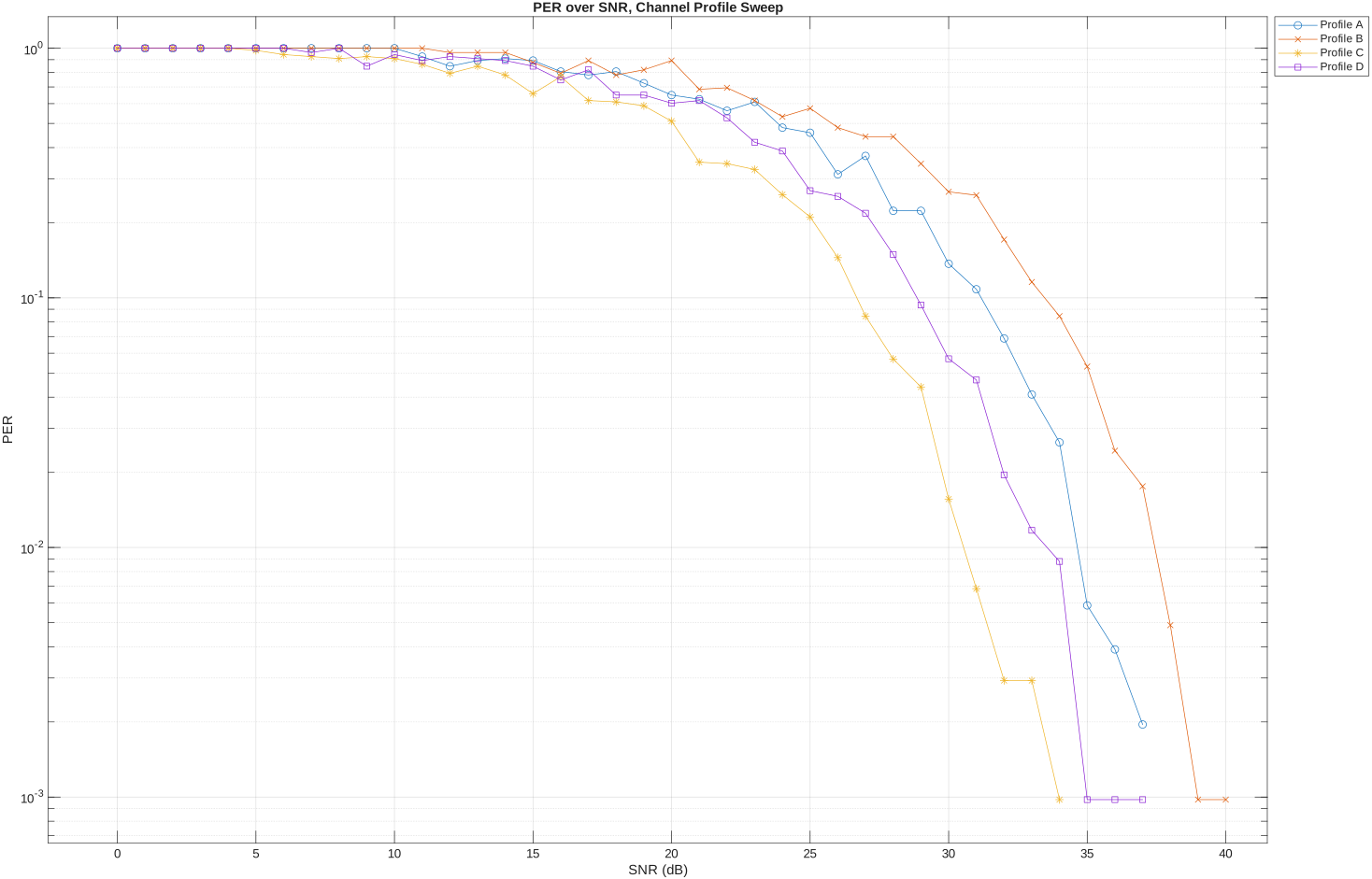 For readability, the labels NTN-TDL-A to NTN-TDL-D are shortened to Profile A to Profile D in the plot. The channel profile sweep shows that the selected NTN-TDL profile has a visible influence on the PER curve. Profile C performs best in this simulation, while Profile B requires the highest SNR for the same target PER. Around the low-PER region, Profile C reaches a PER of approximately $10^{-3}$ about 5 dB earlier than Profile B. Profiles D and A lie between these two cases, with roughly 1-3 dB spacing between neighboring curves for PER values below $10^{-1}$. This means that the channel profile changes the effective link robustness even though all other baseline parameters are kept constant. The difference is caused by the different multipath and fading behavior represented by the NTN-TDL profiles. #### 5.2 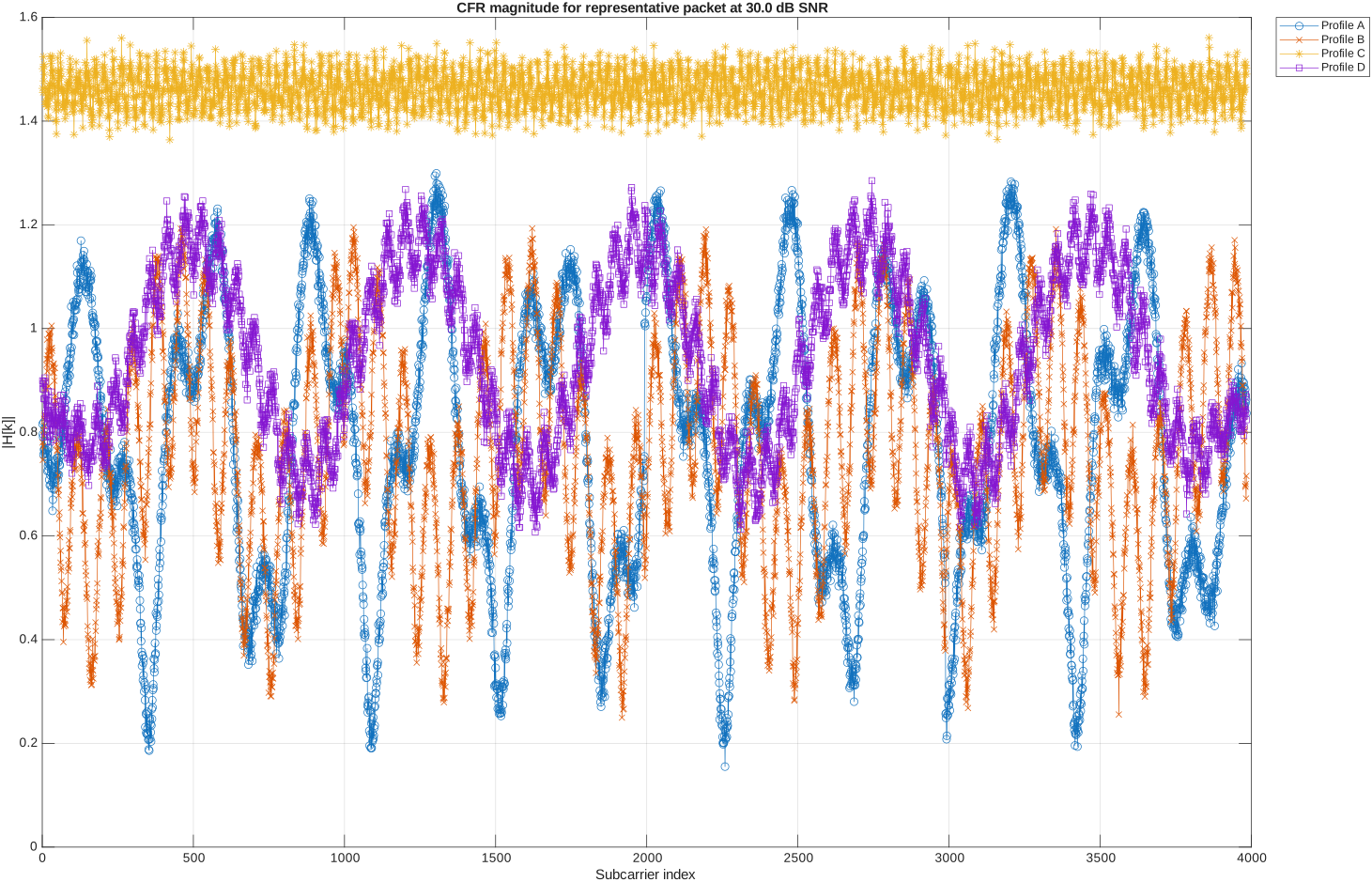 The CFR comparison shows that the NTN-TDL profiles create different frequency-selective channel responses. Profile C has the flattest and highest CFR magnitude at around 1.4 to 1.6 over the active subcarriers, which means that the subcarriers experience a relatively uniform channel gain without strong frequency-selective fades. This is consistent with the PER sweep from Task 5.1, where Profile C performs best. Profiles A and B show stronger variations and deeper periodic fades over the subcarrier range. These fades reduce the effective SNR on parts of the OFDM spectrum and can therefore increase the packet error probability. Profile D lies between these cases, with visible but more moderate frequency-selective behavior. Since this plot shows only one representative packet at 30 dB SNR and 320 MHz bandwidth, it should be interpreted qualitatively. It illustrates how the different channel profiles affect the frequency response, while the PER sweep provides the statistical performance comparison. [This tasks (5.2) interpretation was mainly made from GPT-5.5, because I was not sure what I should assume from the data, after evaluating what GPT interpeted, it made sense and I can see / evaluate the meaning behind the plot]