by Timo Niemann
### Task1 #### 1.1 See code `lab_5.m` and `create_satellite_sim.m`, where the first file defines all parameters for the simulation and the create_satellite_sim function creates and returns the satellite and ground station. #### 1.2 To calculate the distance to the satellite, the MATLAB access analysis example was used as a basis and modified. The distance is calculated with the `aer` function, which returns azimuth, elevation, and slant range between the ground station and the satellite. To avoid invalid channel simulations, the signal-based estimation step is skipped when the Doppler shift `fshift` is non-finite.  The first satellite flyby occurs at around 08:05:30. During the pass, the distance first decreases as the satellite approaches the ground station and then increases again after the closest approach. Around 08:53:30 to 08:54:00, the distance reaches a maximum because the satellite is on the far side of its orbit relative to the ground station. The second pass occurs at around 09:42. Its minimum distance is larger than during the first pass because Earth's rotation changes the relative position of the ground station below the satellite orbit. #### 1.3  As in the distance plot, the elevation angle reaches its highest value during the first pass. The second pass has a lower maximum elevation because Earth's rotation shifts the ground station relative to the satellite ground track. ### Task2 #### 2.1 The normalization calculation is done by firstly extracting the `Short Training Field` from the generated WLAN Waveform: ```matlab tx = wlanWaveformGenerator(txPSDU, cfgEHT); stf = tx(ind.LSTF(1):ind.LSTF(2), :); ``` On the extracted STF the mean of the per value absolute potentiation by 2 is calculated to get the power of the STF: ```matlab stfPower = mean(abs(stf(:)).^2); ``` Following [wikipedia](https://en.wikipedia.org/wiki/DBm) to convert Watt (P) into dBm (x) following formula is used: $x = 10 \cdot \log_{10}\frac{P}{1\text{mW}}$ $= 10 \cdot \log_{10}(P \cdot 1000)$ To simplify that: $= 10 \cdot (\log_{10}(P) + \log_{10}(1000))$ $= 10 \cdot \log_{10}(P) + 10 \cdot \log_{10}(1000)$ $= 10 \cdot \log_{10}(P) + 10 \cdot 3$ $= 10 \cdot \log_{10}(P) + 30$ After this the formula is solved for P, because the MATLAB signal has to be scaled with a linear power value in Watt: $x = 10 \cdot \log_{10}(P) + 30$ $x - 30 = 10 \cdot \log_{10}(P)$ $\frac{x - 30}{10} = \log_{10}(P)$ $10^{\frac{x - 30}{10}} = P$ The `10^` is used because it is the inverse function of `log10`. The division by 10 is needed because the logarithm was multiplied by 10 in the dBm formula. For example, 20 dBm results in: $P = 10^{\frac{20 - 30}{10}} = 10^{-1} = 0.1\text{W}$ The waveform itself is scaled by amplitude and not directly by power. Since power is proportional to the squared amplitude, the scaling factor has to use the square root. Therefore the target power in Watt is divided by the measured STF power and the square root is applied: ```matlab tx = tx * sqrt(10^((txPower - 30) / 10)) / sqrt(stfPower); ``` With this calculation the generated waveform is normalized by the STF power and then set to the desired transmit power in dBm. #### 2.2 To include free space path loss the corresponding field in `create_baseline_configuration.m:37` is set. Following [wikipedia](https://en.wikipedia.org/wiki/Free-space_path_loss)'s free space path loss in decibels, the formula is: $FSPL(dB) = 20 \cdot \log_{10}(\frac{4\pi d}{\lambda})$, where $\lambda = \frac{c}{f}$ Therefore the wavelength is calculated from the carrier frequency: ```matlab lambda = physconst("lightspeed") / carrier_frequency; ``` The received power is then the transmit power minus the free space path loss: $P_{rx} = P_{tx} - FSPL$ This is possible because `P_tx` and `P_rx` are dBm values, while `FSPL` is a dB loss. In the simulation this is implemented as: ```matlab pathLoss(numPacketsSimulated) = 20 * log10(4 * pi * packetDistance / lambda); rxPower(numPacketsSimulated) = txPower - pathLoss(numPacketsSimulated); ``` 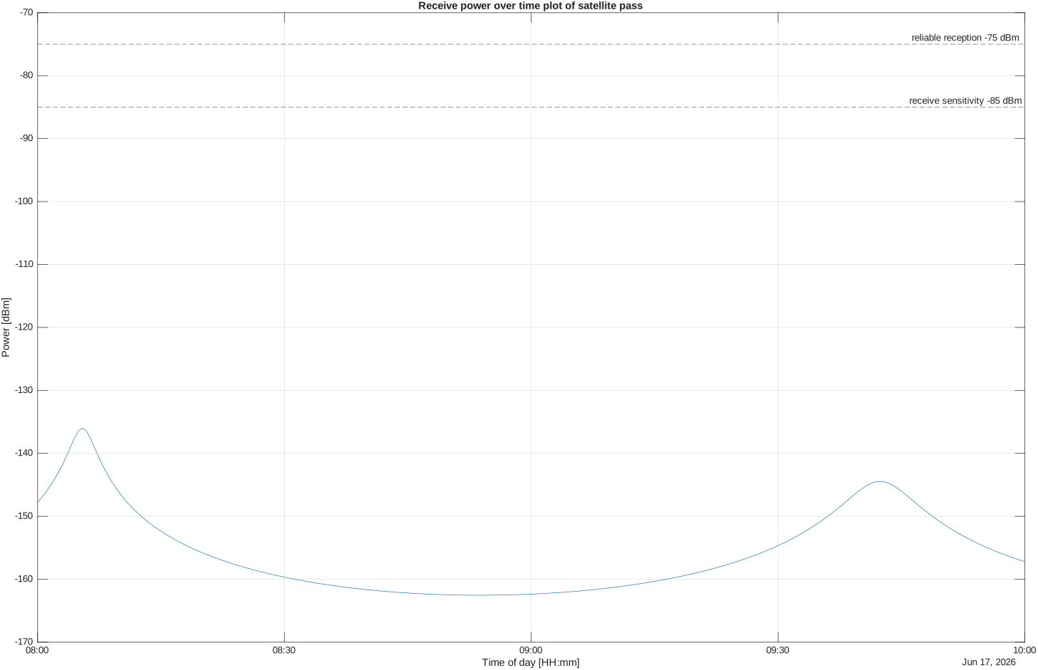 #### 2.3 [calculatorshub.net](https://calculatorshub.net/telecom-calculators/dbm-to-range-calculator/) - this site provided helpful formulas and verification possibilities. A signal is detectable when the receive power has at least a sensitivity of -85 dBm: $P_{rx} \geq -85dBm$ The simulated receive power is below this threshold during the whole satellite pass. With the normal 20dBm WiFi transmit power, the received signal is therefore not detectable by a typical WiFi node. To calculate the maximum reachable distance for detectability, the free space path loss formula is used in the opposite direction. With a transmit power of 20 dBm, the maximum allowed path loss is: $FSPL_{max} = P_{tx} - P_{rx}$ $FSPL_{detectable} = 20dBm - (-85dBm) = 105dB$ The free space path loss formula is then solved for the distance `d`: $FSPL = 20 \cdot \log_{10}(\frac{4\pi d}{\lambda})$ $\frac{FSPL}{20} = \log_{10}(\frac{4\pi d}{\lambda})$ $10^{\frac{FSPL}{20}} = \frac{4\pi d}{\lambda}$ $d = \frac{\lambda}{4\pi} \cdot 10^{\frac{FSPL}{20}}$ This is why the code calculates: ```matlab maxPathLossDetectable = txPower - wifiSensitivity; maxDistanceDetectable = lambda / (4 * pi) * 10^(maxPathLossDetectable / 20); ``` The calculation results in a maximum detectable distance of 1.77km with 20dBm transmit power. This is much smaller than the satellite distance during the pass, so a normal WiFi transmit power is not sufficient for this link. #### 2.4 To calculate the required transmit power for reliable reception, the receive power formula is solved for `P_tx` instead: $P_{rx} = P_{tx} - FSPL$ $P_{tx} = P_{rx} + FSPL$ For reliable WiFi reception the target receive power is -75 dBm. Therefore the required transmit power is: $P_{tx,required} = -75dBm + FSPL$ With normal 20dBm transmit power, this reliable reception threshold would only allow a maximum distance of 0.56km: ```matlab maxPathLossReliable = txPower - reliableRxPower; maxDistanceReliable = lambda / (4 * pi) * 10^(maxPathLossReliable / 20); ``` In MATLAB this is: ```matlab requiredTxPower = reliableRxPower + pathLoss; ``` 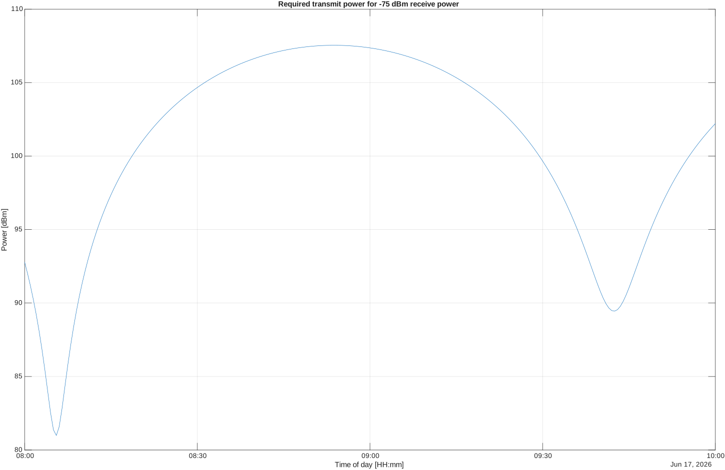 For the simulated satellite pass, the required transmit power for -75dBm receive power is between 80.99dBm and 107.54dBm. This is far above the normal 20dBm WiFi transmit power. #### 2.5 The transmit amplifier can add 30 dB gain. Together with the original 20 dBm transmit power, the amplified transmit power is: $P_{tx,amplified} = 20dBm + 30dB = 50dBm$ If the required transmit power is still higher than this value, the missing difference has to be provided as antenna gain: $G_{antenna} = P_{tx,required} - P_{tx,amplified}$ Negative antenna gain is not needed, therefore the value is limited to zero: ```matlab amplifiedTxPower = txPower + amplifierGain; requiredAntennaGain = max(requiredTxPower - amplifiedTxPower, 0); ``` With the 30dB amplifier, the remaining required antenna gain is between 30.99dB and 57.54dB.